Dijkstra’s Algorithm | Code and Examples Walkthrough
Shortest path problems show up everywhere in computing.
Shortest path problems show up everywhere in computing. Whenever you want to find the cheapest route from one place to another in a network with costs on the edges, you are solving a shortest path problem. That might be a map with driving times, a network of servers with latency, or a game world where an agent needs to move around obstacles efficiently.
What’s the Point?
Imagine you have a directed graph where each edge has a cost. You pick a starting node and you want to know the smallest possible total cost to reach every other node in the graph. You do not just want any path. You want the cheapest path according to the sum of edge weights.
Brute forcing all possible paths would be incredibly expensive for anything larger than toy examples. Dijkstra’s algorithm uses a greedy strategy that explores the graph in a smart order and keeps track of the best distances found so far. It assumes that all edge weights are non-negative. Under that assumption, when the algorithm says a node has distance 5, it can guarantee that no other path from the start to that node will ever produce a smaller value later.
A High Level Overview
Start with a weighted graph where edges have non-negative costs and choose a starting node. Set the distance to the start node as 0 and set the distance to every other node as infinity to represent “unknown” distance.
Keep a distance table that stores the best known distance from the start to each node. Alongside that, keep a priority queue that always gives you the node with the smallest current distance.
Insert the start node into the priority queue with distance 0. All other nodes stay out of the queue until the algorithm finds some path to them.
While the priority queue is not empty, remove the node with the smallest distance. Think of this as the frontier of the wave of shortest paths.
If this node has already been processed before, skip it. Otherwise mark it as finalized, meaning its current distance is now guaranteed to be the true shortest distance from the start.
Look at all neighbors you can reach directly from this node. For each neighbor, compute a candidate new distance equal to the current node’s distance plus the weight of the edge to that neighbor.
If this candidate distance is smaller than the neighbor’s recorded distance in the table, update the neighbor’s distance to this new, better value and push the neighbor into the priority queue with that updated distance. This is the relaxation step.
Repeat the process: always pull the closest unfinished node from the priority queue, finalize it, and relax its outgoing edges. Because all edge weights are non-negative, once a node is finalized its distance will never improve later.
When the priority queue becomes empty, every reachable node has been finalized. The distance table now holds the shortest path cost from the starting node to every other node in the graph.
Our Code Implementation
Our implementation takes a NetworkX directed graph and a starting node, and returns a dictionary that maps each node to its shortest distance from the start.
import heapq
import networkx as nx

“”“
In Python, there are many ways to represent a graph.
For this article, we will use NetworkX because it
provides a clean interface for working with nodes and edges
and lets us attach the weights directly to edges.

Example weighted directed graph:

G = nx.DiGraph()
G.add_weighted_edges_from([
    (”A”, “B”, 4),
    (”A”, “C”, 1)
])

Each tuple is (source, target, weight), and the weight can be accessed as:

weight = G[”A”][”B”][”weight”]
“”“

def dijkstra(graph, start):

    # STEP 1: Initialize distances
    # --------------------------------
    # We create a distance table where every node starts at infinity.
    # Infinity means “unknown” or “unreachable” at the beginning.
    # The start node is set to 0 because the distance from the start
    # to itself is zero.
    distances = {node: float(”inf”) for node in graph.nodes()}
    distances[start] = 0

    # STEP 2: Set up the priority queue (min heap)
    # --------------------------------
    # We use a priority queue to always expand the node with the
    # smallest known distance so far.
    # Each entry in the queue is a pair (distance, node).
    # We begin with just the start node at distance 0.
    pq = [(0, start)]

    # STEP 3: Track which nodes have been finalized
    # --------------------------------
    # Once we “visit” a node and accept its shortest distance,
    # we add it to the visited set. After that, we will not
    # try to relax edges from this node again.
    visited = set()

    # STEP 4: Main loop of the algorithm
    # --------------------------------
    # While there are still nodes in the priority queue:
    #   1. Pop the node with the smallest distance.
    #   2. If it is already visited, skip it.
    #   3. Otherwise, treat its distance as final and relax its edges.
    while pq:
        current_dist, node = heapq.heappop(pq)

        # If we have already processed this node with a better distance,
        # then this entry is outdated and we skip it.
        if node in visited:
            continue

        # Mark this node as finalized. Its distance in the table
        # is now the best possible.
        visited.add(node)

        # STEP 5: Relax edges from the current node
        # --------------------------------
        # For each neighbor reachable from this node, we consider
        # using the path that goes through the current node.
        # If that path gives a better distance than what we have
        # stored, we update it and push the neighbor into the queue.
        for neighbor in graph.neighbors(node):
            weight = graph[node][neighbor][”weight”]
            new_dist = current_dist + weight

            # Relaxation step:
            # If going through “node” gives a shorter distance to “neighbor”,
            # update the neighbor’s distance and push it back into the heap.
            if new_dist < distances[neighbor]:
                distances[neighbor] = new_dist
                heapq.heappush(pq, (new_dist, neighbor))

    # STEP 6: Return the final distance table
    # --------------------------------
    # At this point, the priority queue is empty and every reachable
    # node has been processed. The “distances” dictionary holds the
    # shortest path distance from the start node to every other node.
    return distances
Example 1:
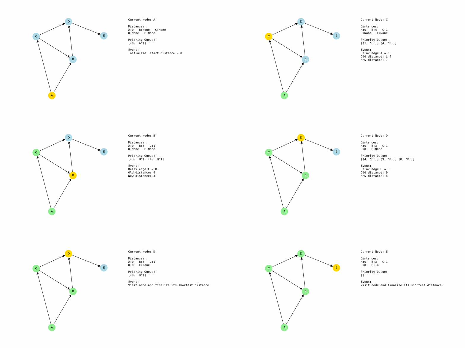
Let us try this implementation on a small graph with five nodes named A, B, C, D, and E. This example is simple enough to reason about by hand, which makes it a good sanity check.
We create the graph and call dijkstra starting from node A…
G1 = nx.DiGraph()
G1.add_weighted_edges_from([
    (”A”, “B”, 4), # A to B with cost 4
    (”A”, “C”, 1), # A to C with cost 1
    (”C”, “B”, 2), # C to B with cost 2
    (”B”, “D”, 5), # B to D with cost 5
    (”C”, “D”, 8), # C to D with cost 8
    (”D”, “E”, 6) # D to E with cost 6
])

dijkstra(G1, “A”)
The distance to A begins at 0 and every other node starts at infinity. From A, there are two outgoing edges: A to B with cost 4 and A to C with cost 1. That gives B a tentative distance of 4 and C a tentative distance of 1. Since C currently has the smaller distance, the priority queue selects C as the next node to process.
From C, there are edges to B with cost 2 and to D with cost 8. If we go from A to C to B, the total cost is 1 + 2 = 3. That is better than the previous distance of 4 for B, so B is updated to 3. For D, the path A → C → D has cost 1 + 8 = 9, so D gets a tentative distance of 9.
At this point, B has distance 3 and D has distance 9, so the algorithm picks B next. From B, there is an edge to D with cost 5. That creates a new candidate distance for D: 3 + 5 = 8. Since 8 is better than the previous 9, D’s distance is improved to 8.
Finally, D is processed at distance 8. From D, there is an edge to E with cost 6, so E receives a distance of 8 + 6 = 14. At the end of the run, the shortest distances from A are: A = 0, C = 1, B = 3, D = 8, and E = 14.
Example 2:
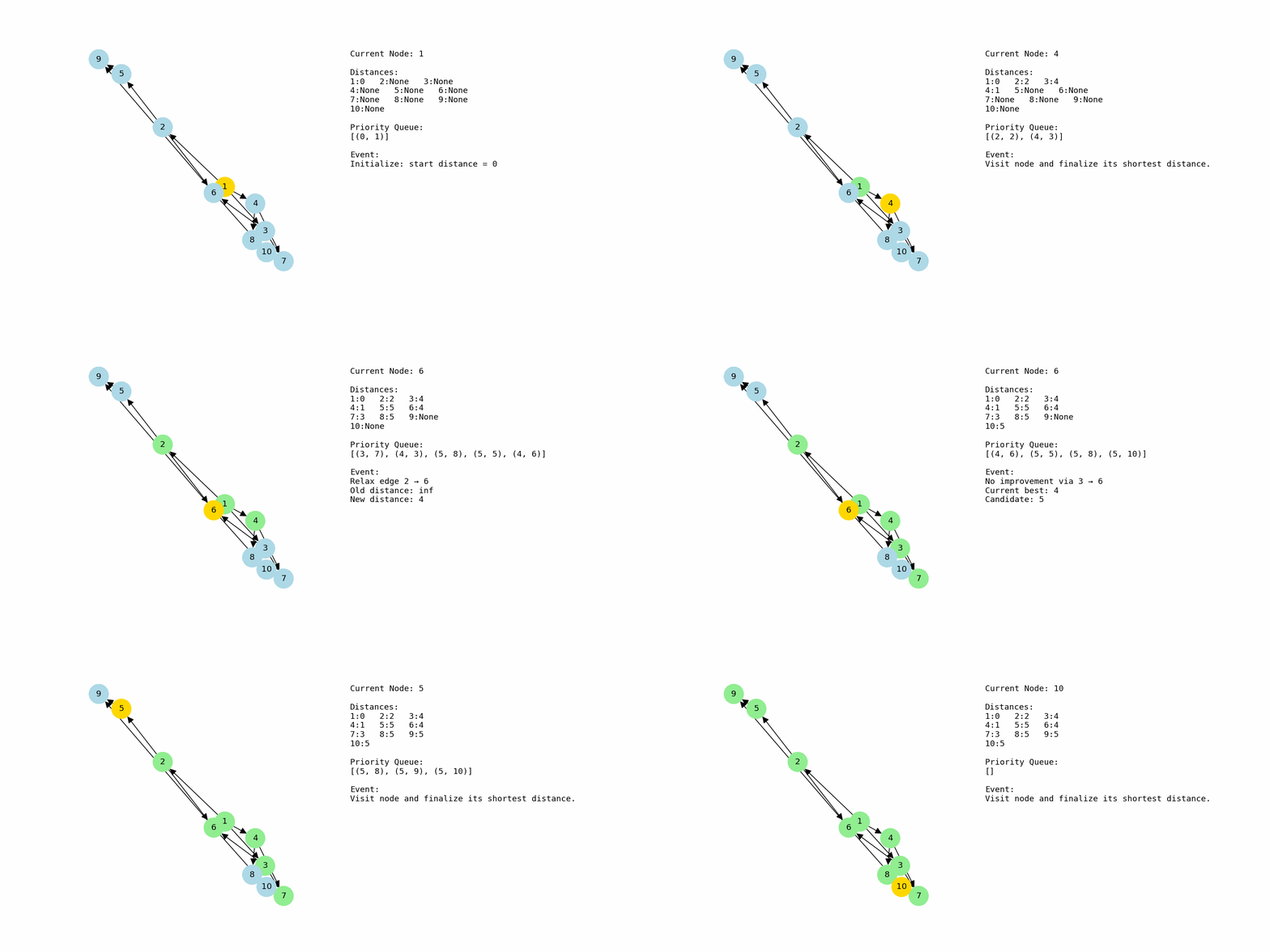
Now let us look at a slightly larger graph where the dynamics of the algorithm become more interesting. This one uses integer node labels from 1 through 10.
We build and call it like this:
G2 = nx.DiGraph()
G2.add_weighted_edges_from([
    (1, 2, 2), (1, 3, 4), (1, 4, 1),

    (2, 5, 3), (2, 6, 2),
    (3, 6, 1), (3, 7, 5),
    (4, 7, 2), (4, 8, 4),

    (5, 9, 4),
    (6, 9, 1), (6, 10, 5),
    (7, 10, 2),
    (8, 10, 3)
])

dijkstra(G2, 1)
Now consider the second example, where the nodes are labeled from 1 to 10 and the graph has more branching paths. The algorithm starts at node 1 with distance 0 and every other node at infinity. From node 1, there are edges to 2 with cost 2, to 3 with cost 4, and to 4 with cost 1. After relaxing these edges, the tentative distances are 2 for node 2, 4 for node 3, and 1 for node 4. Node 4 is currently the closest, so it is chosen next.
From node 4, the algorithm sees edges to 7 with cost 2 and to 8 with cost 4. This results in distance 3 for node 7 (1 + 2) and distance 5 for node 8 (1 + 4). At the same time, node 2 is still sitting in the priority queue with distance 2, so it will be processed soon. When node 2 is selected, its edges to 5 and 6 are relaxed, giving node 5 a distance of 5 (2 + 3) and node 6 a distance of 4 (2 + 2). Now the frontier contains nodes 3, 6, 7, 8, and 5 with various tentative distances.
Node 7 currently has distance 3, which is smaller than the distances of 3, 5, 6, and 8, so it is processed next. From node 7, there is an edge to node 10 with cost 2, so node 10 gets a tentative distance of 5 (3 + 2). After that, node 3 is processed with distance 4, but its outgoing edges only produce distances that are not better than the ones already stored for nodes 6 and 7, so no updates are made. Node 6 is then processed with distance 4. From node 6, relaxing the edge to node 9 yields a new distance of 5 (4 + 1). The path through 6 to 10 would cost 9, which is worse than the existing 5 for node 10, so node 10 is not updated.
Finally, the algorithm processes the remaining nodes that sit at distance 5, such as 5, 8, 9, and 10. None of their outgoing edges can improve any distances further, so the table stabilizes. The final shortest distances from node 1 are: 1 = 0, 2 = 2, 4 = 1, 7 = 3, 3 = 4, 6 = 4, and 5, 8, 9, and 10 all at 5. This example shows how Dijkstra smoothly handles multiple competing routes and converges on the minimum distances without needing to explore every possible path explicitly.
Try Reasoning it Yourself!
G3 = nx.DiGraph()

G3.add_weighted_edges_from([
    (1, 2, 4), (1, 3, 2), (1, 4, 5),

    (2, 5, 3), (2, 6, 2),
    (3, 6, 4), (3, 7, 1),
    (4, 7, 2), (4, 8, 6),

    (5, 9, 5), (5, 10, 3),
    (6, 10, 2), (6, 11, 6),
    (7, 11, 3), (7, 12, 4),
    (8, 12, 2), (8, 13, 7),

    (9, 14, 3),
    (10, 14, 1), (10, 15, 6),
    (11, 15, 2), (11, 16, 5),
    (12, 16, 3),
    (13, 16, 4)
])

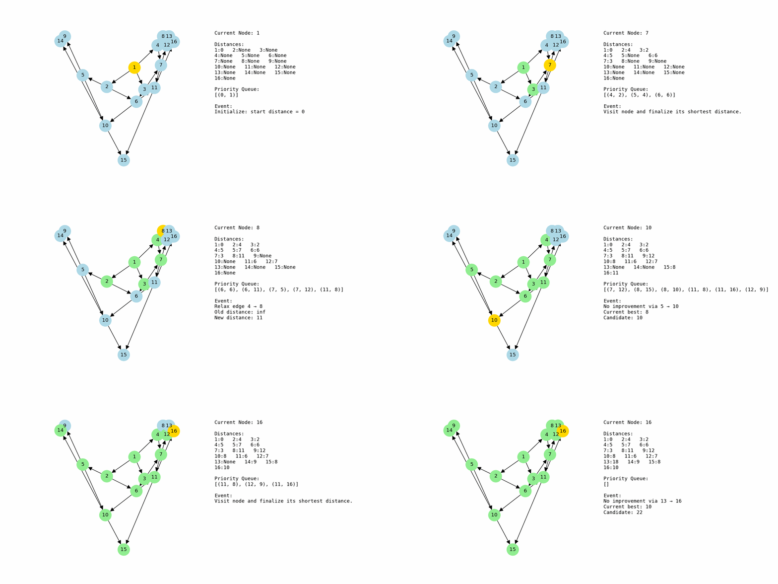
dijkstra_with_gif(G3, 1, “example3_large.gif”)


